
I just finished watching The Great Flood last night and me and my mom started talking about it and that conversation led to her AI fear-mongering coming out. Good movie though overall based around what I perceived to be model training and I was studying the basics of that not too long ago and what better way to learn than to teach. Also most of this comes from google and they also go more into depth if you want to check it out as well, not like they need me to grift for them LOL.
Where it all starts
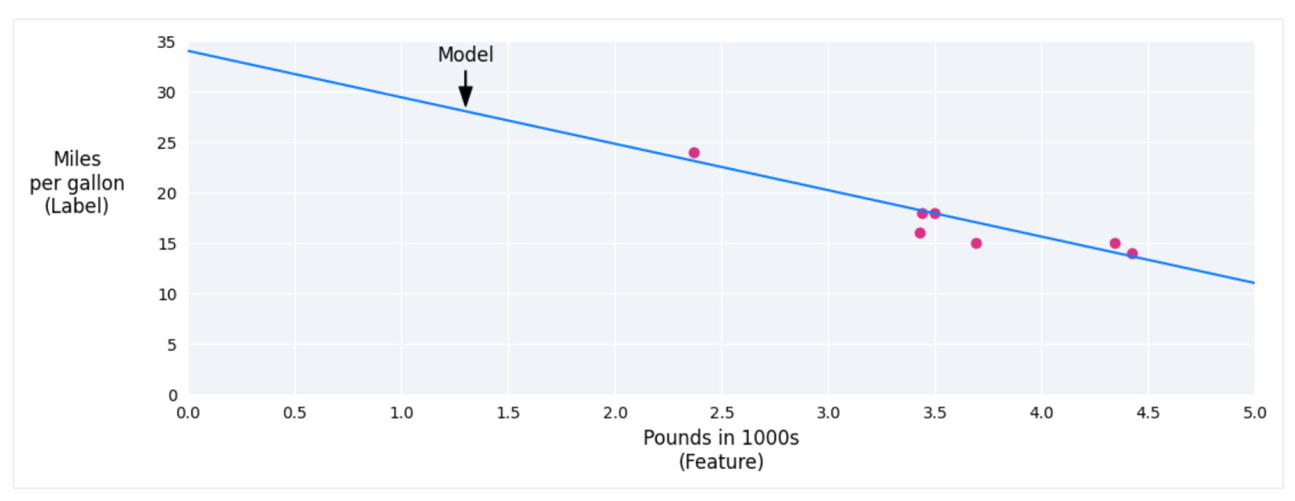
Linear regression is a statistical technique used to find the relationship between variables and in a machine learning context, the relationship between features and labels. You can think of it as plotting all the points on the graph and drawing a best fit line of all the points.
For example we have a dataset and we want to plot the data to make a best fit line.
Let's get the basics out of the way
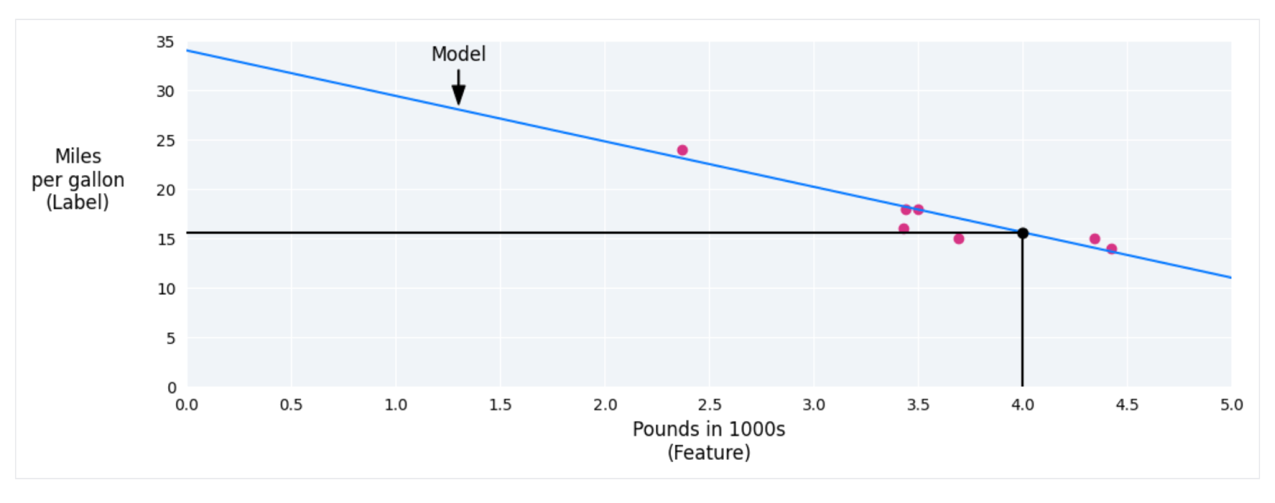
The equation for linear regression in a machine learning context is defined as:
= Predicted label, also the output.
= Bias. Same concept as the y-intercept and is calculated during training.
= Weights of the feature. Same as the slope and is calculated during training.
= feature, also the input.
What happens when there’s more than one feature?
Obviously something more advanced has multiple features but the regression formula is similar even when each feature has a different weight. For example if a model has 5 features each with a different weight:

More data = better information the model can go off of (potentially, it really depends on quality of the data)
Now onto the loss of a model
The loss is a metric that pretty much describes how wrong the model’s predictions are. When training a model and graphing its predictions against the actual values, the loss is the distance between the two. When we’re training the model our goal is to pretty much minimize this value as much as possible. When training it’s always best to average out the loss over all of the examples rather than just taking a few.
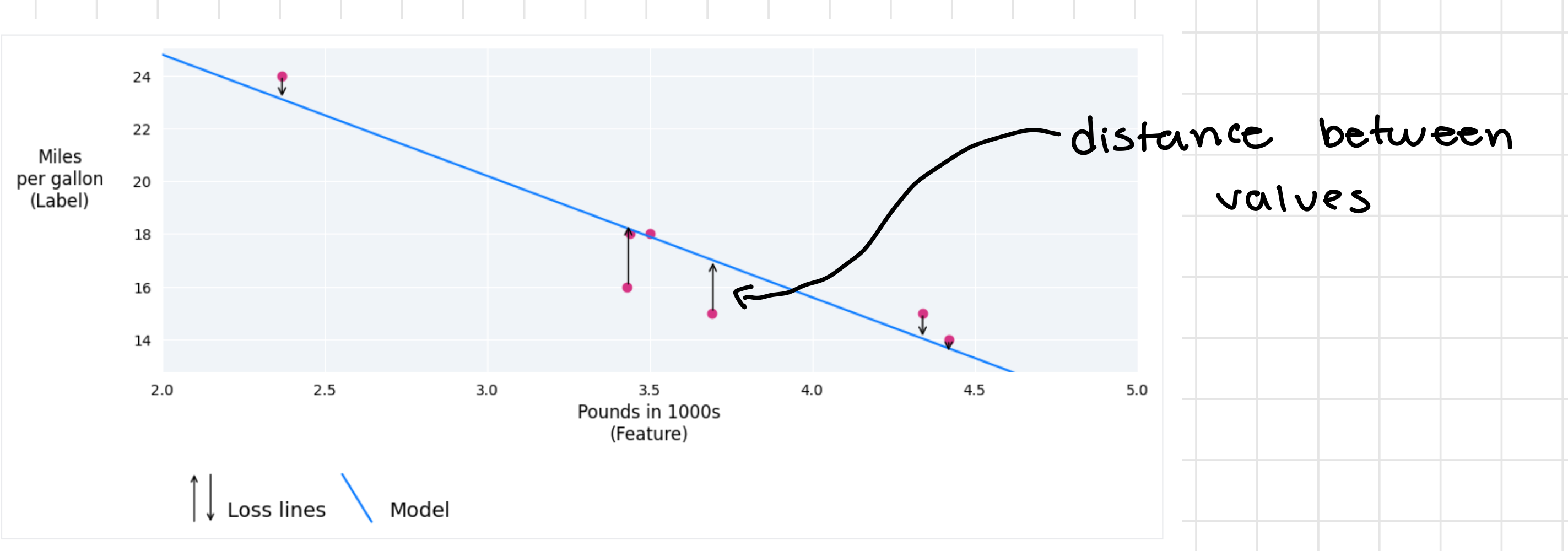
Distance of Loss
The loss focuses on the distance between the values and not the direction. To do this we have two common methods to get this value:
- Take the absolute value.
- Square the difference between the actual value and the predicted value.
That brings us to the different types of loss
In linear regression we have 5 main types of loss (av = actual value , pv = predicted value):
| Loss Type | Definition | Equation |
|---|---|---|
| loss | the sum of absolute values of the difference between the predicted value and the actual value. | |
| Mean Absolute Error (MAE) | the average of loss over a set of N examples. | |
| loss | sum of squared differences between the predicted value and the actual value. | |
| Mean Squared Error (MSE) | the average of loss over a set of N examples. | |
| Root Mean Squared Error (RMSE) | the square root of mean squared error. |
The functional difference between and loss is how the error is weighted. When the difference between the values is big, using loss and squaring makes the error bigger, when the difference is small (error < 1), loss makes the error even smaller.
Mean Squared Error or Root Mean Squared Error are usually the more preferred type for loss since they’re expressed in the same units that you give them and don’t need to deal with cursed squared units.
Calculating Loss
We can give a quick example of how calculating the loss of a model would work for loss:
| Value | Equation | Result |
|---|---|---|
| prediction | bias + (weight * feature) | Predicted Value |
| actual value | label | actual value |
| loss | (actual value - predicted value) | loss value |
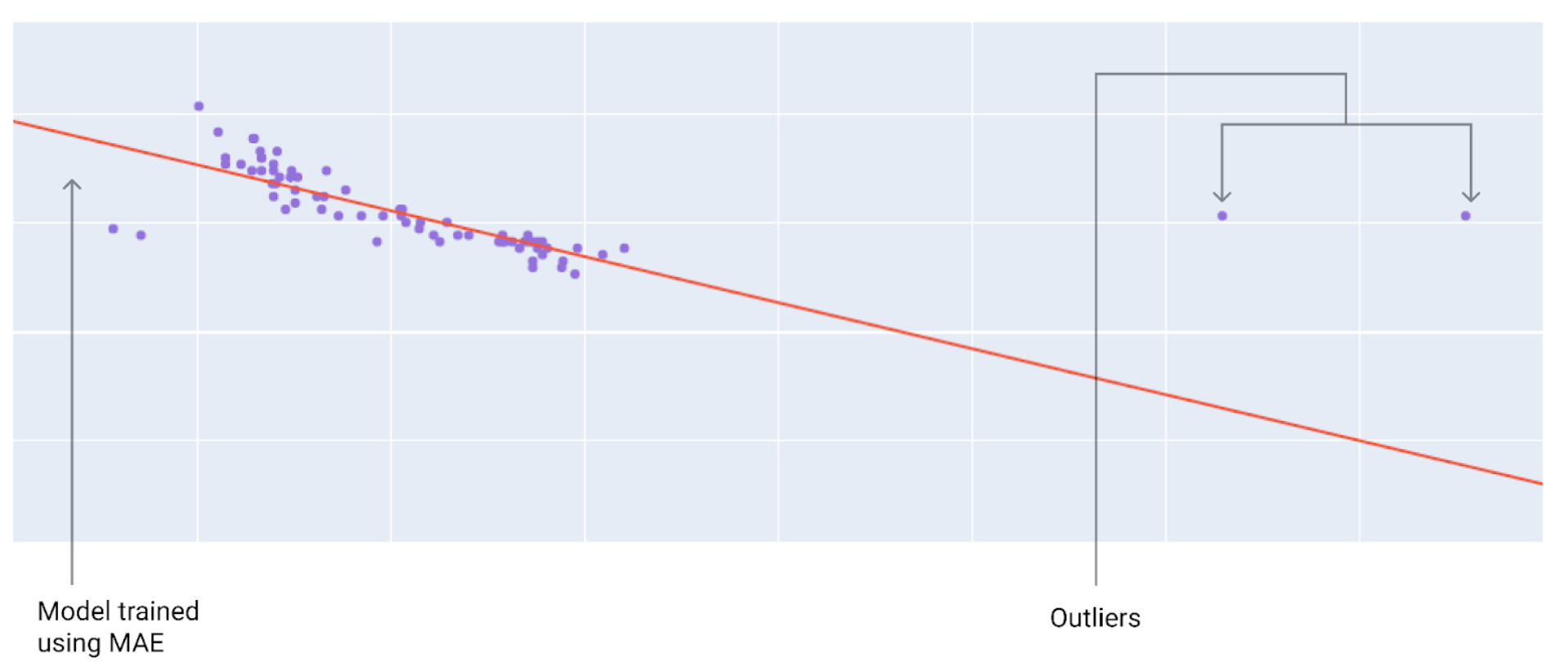
Choosing a loss
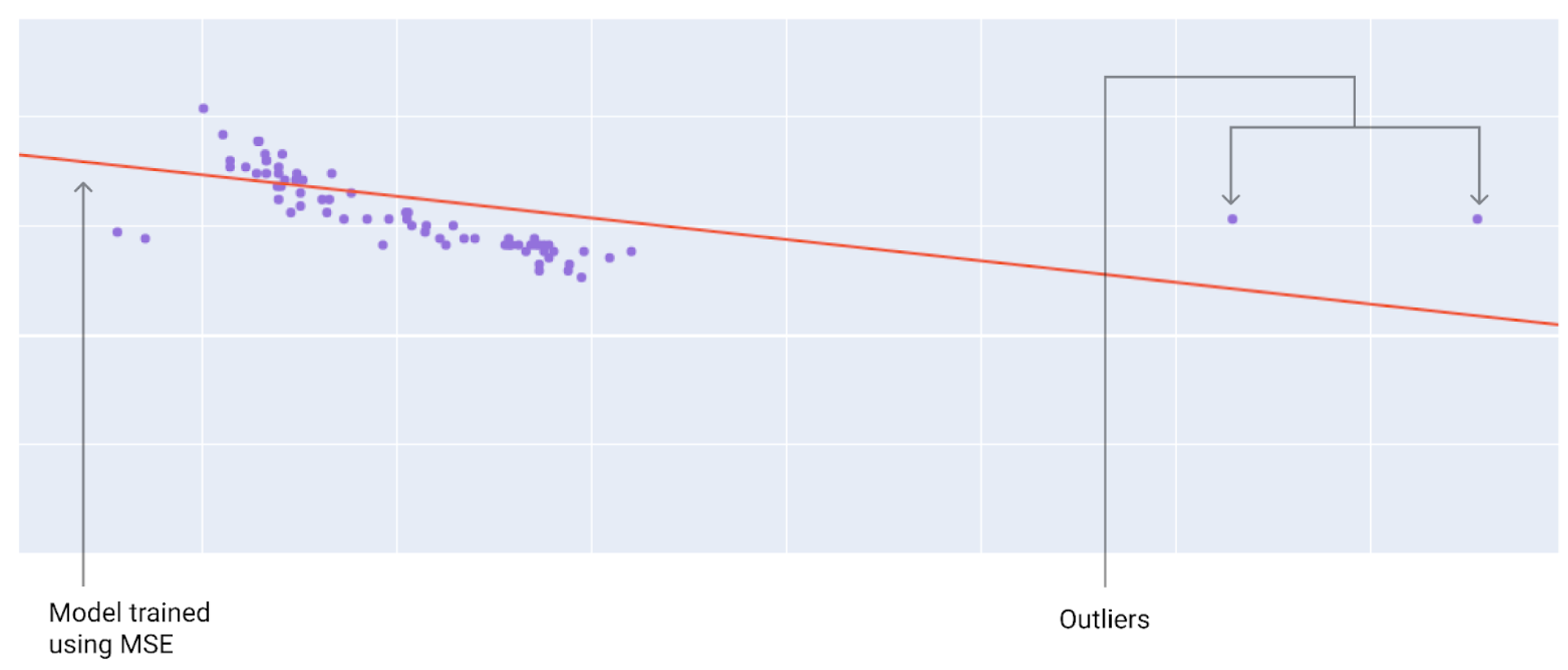
Choosing between MAE or MSE or any other type of loss really just depends on your data and how you want it to handle certain predictions and outliers. Using MSE or loss, the model moves towards outliers. Using MAE or loss, the model moves closer to the average of all the data. For an easy to remember relationship, squaring moves towards outliers and absolute values don’t.
One of the most important algorithms
Gradient descent (maybe the most important algorithm, hot take) is a technique in math that iteratively finds the weights and bias for a function that gives the model with the lowest loss value. When we first start training the model, we start with the weights and bias with an initial value set close to 0 and repeat the following steps:
- Calculate loss with the current weights and bias.
- Determine the direction to move the weights/bias to reduce the amount of loss.
- Move the weights and bias a small amount in the determined direction to reduce the loss.
- Return to step 1 and repeat until the model can’t reduce the loss further
For a more technical breakdown (because why not):
-
We start with the initial values of the weights and bias set to 0.
weights = 0 , bias = 0 , y = w() + b
-
We calculate the loss with the current model parameters. For example using Mean Squared Error we can use the formula we saw above (after this were going to use proper notation so people don't attack me lol).
-
To get the tangent (slope) of the loss function at each weight and bias.
To get the tangent for both the weight and the bias we have to take the partial derivative of the loss function with respect to both the weights and also for the bias.
Lets say we have our equation for making our prediction from above:
we can represent the above equation with
y.wandbwill represent our weights and bias andxis our input value.The partial derivative of the loss function with respect to the weight is written as:
Where all instances of the bias are treated as a constant and once differentiated the formula evaluates to:
Solving this equation with a weight and a bias we can get a slope that we’ll define as
Similarly, the partial derivative of the loss function with respect to the bias is written as:
In this case all instances of the weight are treated as constants when differentiating the equations and evaluates to
Solving this equation with a weight and a bias we can get a slope we’ll define as
-
We move a small amount in the direction of the negative slope to get to the next weight and bias to evaluate. We can define the learning rate as some arbitrary value, for example 0.01.
new weight = old weight - (0.01 * )
new bias = old bias - (0.01 * )
we use the new weight and bias to calculate the loss and the repeat the process until the value converges and we have the weights and bias that minimize the loss the most.
Model Convergence and Loss Curves
When we’re training a model we look at the loss curves to see if the model has converged or is actually learning in its training. It shows us how the loss of the model changes as it’s training which can quickly let us know how bad our initial parameters were.
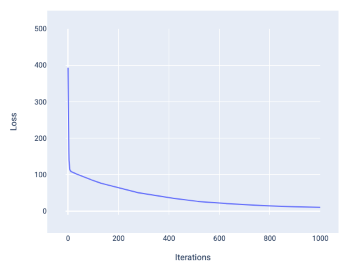
In the above example it shows that the model converges after around 1000 iterations. The loss initially goes down significantly but then flattens out later down the graph which shows the relations between the weights, bias and loss all converging and going to a minimum.
Convergence and convex functions
Loss functions for linear models always produce convex surfaces, which has a property that when the linear regression model converges we know we have found the weights and bias with the lowest loss. Graphing the loss surface for a model with one feature we see the weights on the x axis, bias on the y axis and loss on the z axis.
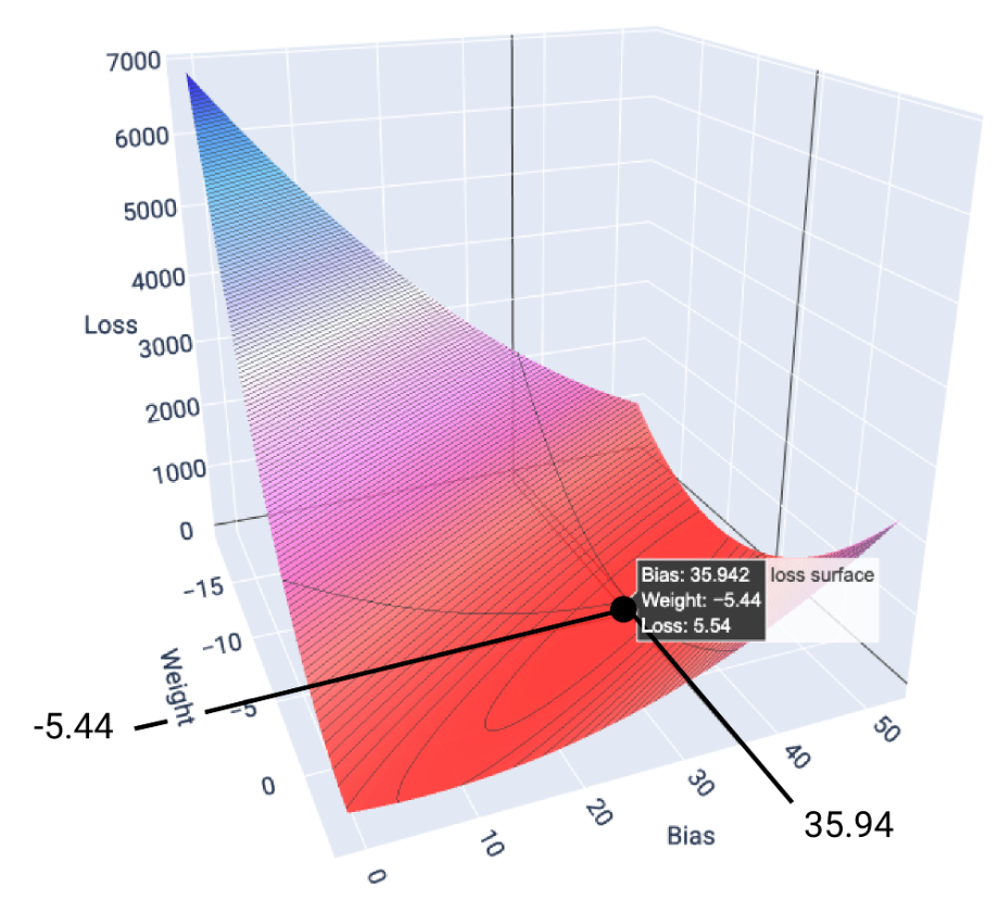
Once it has converged to the minimum point we have found the ideal weight and bias for minimum loss. Minimum loss does not mean zero loss but for the given parameters, its the lowest loss thats attainable.
Hyperparameters
Hyper Parameters are the variables that control the different aspects of training a model. Three common hyperparameters are:
- Learning rate
- Batch size
- Epochs
Learning Rate
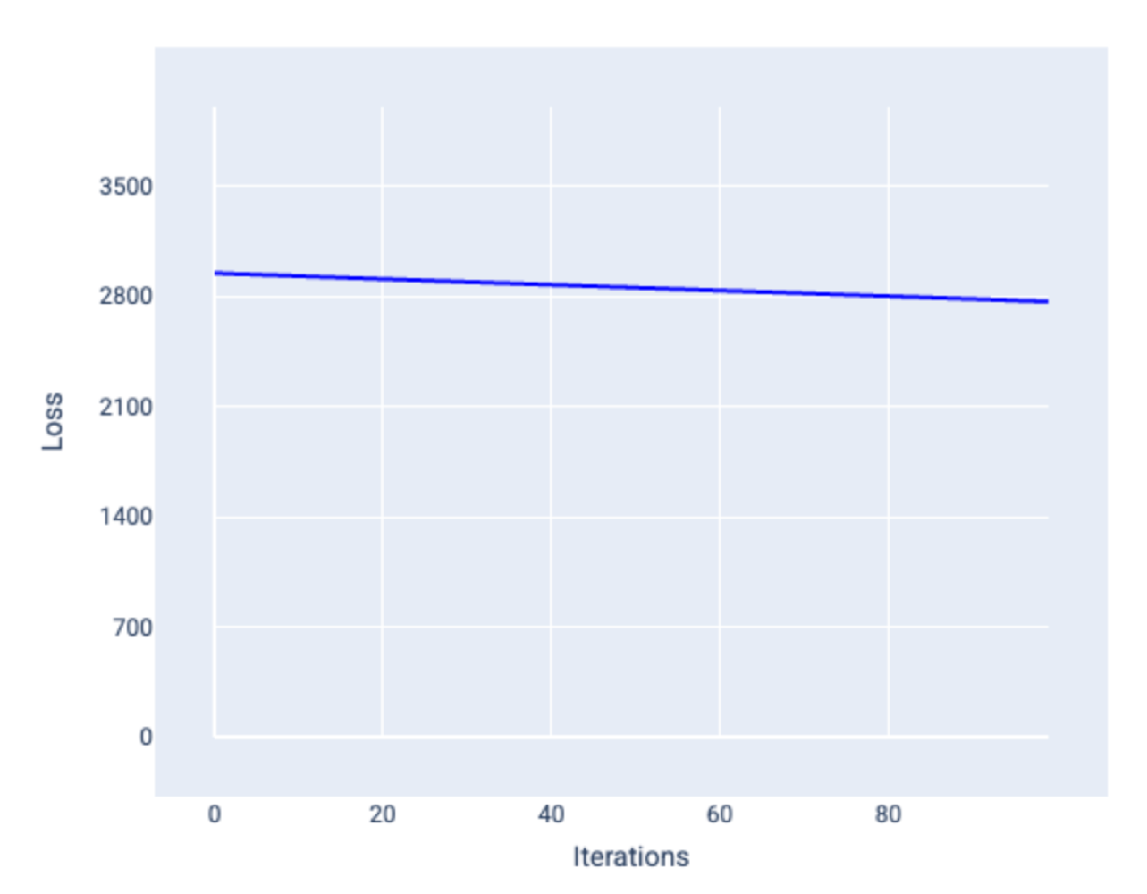
Learning rate is a floating point number that influences how fast the model converges. With a lower learning rate the model may take too long to converge, if too high the model will never converge and just continues to bounce around. The learning rate determines the magnitude of change to make to the weight and bias during each step of gradient descent. The “small amount” discussed in gradient descent refers to the learning rate and an ideal learning rate helps the model converge in a reasonable amount of steps
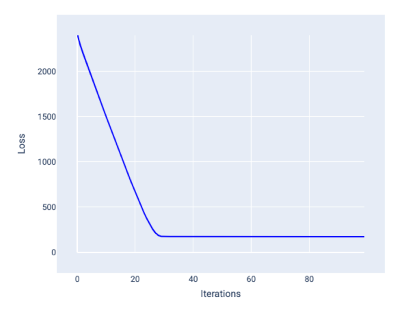
Small learning rate that takes too many iterations to converge.
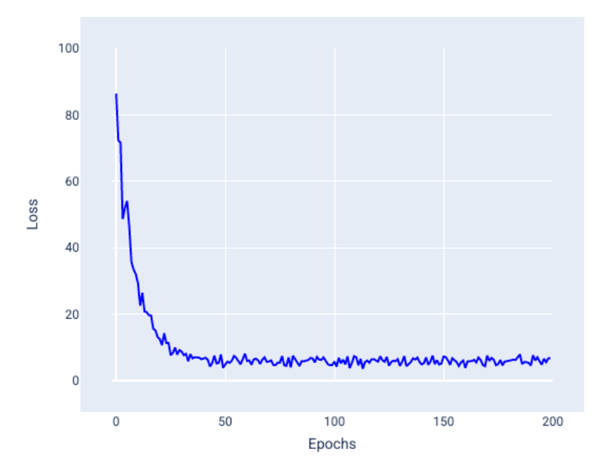
Learning rate that converges quickly.

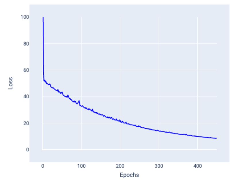
Learning rate too high that the value jumps around and never converges as iterations increase.
Batch Size
Batch size is the number of examples the model processes before updating its weights and biases. Sometimes when datasets contain hundreds of thousands or millions of examples, using the entire batch isn’t always practical. There are 2 common techniques to get the right gradient on average without having to look at every example in the dataset:
- Stochastic gradient descent
- Mini-batch stochastic gradient descent
Stochastic Gradient Descent
SGD uses only a single random example (batch size = 1) for each iteration. With enough iterations it works but it can be very noisy throughout the entire loss curve and the loss may increase instead of decrease on an iteration. Below is a loss curve of SGD.
Mini-batch Stochastic Gradient Descent
Mini-batch SGD is a compromise between full batch and SGD. for any N points the batch size can be 1 < x < N. The model chooses the examples for each batch at random and averages their gradients and updates the weights and bias once per iteration of all examples in the batch. Smaller batch sizes behave like normal SGD and larger ones behave like full batch gradient descent. The noise is not always a bad thing and sometimes it can help the model generalize and find the optimal weights and bias. Below is a loss curve of using mini-batch SGD.
Epochs
In training a model, an epoch means that the model has processed every example in the training set once. For example, if a training set has 1,000 examples and each mini-batch size is 100 examples, it’ll take 10 iterations to complete one epoch. Usually a model has to go many epochs to finish its training and the number of epochs is a hyper parameter set before the model begins training. In general, the more epochs produces a better model but it can also take more time to train.
This is just a super basic introduction into linear regression and I just wanted to put this out there and maybe it’ll help someone understand these concepts a bit better and kick off their own learning. Happy New Year, everyone, cheers.